Stereo Image Rectification

Project Overview

Stereo vision refers to processing of images from two cameras that are placed relative to each other at a known configuration. The two separate but similar views obtained from each individual camera can be used to compare pixels in both images and triangulate the scene’s depth. Stereo image rectification projects images onto a common image plane in such a way that the corresponding points have the same row coordinates. This image projection makes the images appear as though the two cameras are parallel.

In this project, I apply stereo rectification to two pairs of stereo images of two separate scenes. These rectified images can be used for depth estimation, which will be done in a subsequent project.

Original Stereo Images

Here the original images are shown with a grayscale operation applied to each. Note each image includes a left and right image taken with a separate camera lens with its own camera center. Using grayscale simplifies the problem to only one channel. The color information from the image is not important as the feature detection and matching relies more on the gradients and geometry present in the scene.

Identifying Key Features

The keypoints are detected in each image. These key features are then used to detect which features are present in both images and how much they have moved. The SIFT algorithm is used using OpenCV for detecting the features and descriptors.

Matching Features Across Images

The FLANN matches is used to match keypoints. It sorts the best potential matches between similar keypoints in both frames based on their distance using a K-nearest-neighbor search. The best keypoints are selected where we are sure they are matched in both images to calculate reprojection matrices.

Epipolar Lines

So far we have done 2D matching in image frame. To get the relationship to 3D real world coordinates, we need to use epipolar geometry. The fundamental matrix gives us the relationship between the two images and maps points of one image to lines in another. The epipolar constraint tells us that a matching pixel in an image is on the epipolar line. This simplifies the search to the epipolar line and saves us from searching the whole image. We draw the epilines on the image.

Rectified Images

Note the epipolar lines are at an angle in both images. Using stereo rectification in OpenCV, we reproject the images to a common plane that is parallel to the line between camera centers. This then gives us the final rectified images.

Code Runtime

Code

				
					# import required libraries
import numpy as np
import cv2 as cv
import matplotlib.pyplot as plt
import time

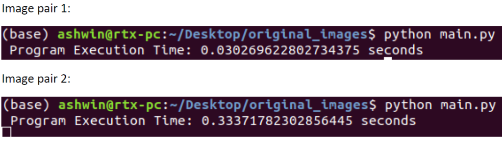
# start timing program execution
start_time = time.time()

# function to draw epilines on our image
def drawlines(left_imgsrc, right_imgsrc, lines, pts1src, pts2src):
    r, c = left_imgsrc.shape
    left_imgcolor = cv.cvtColor(left_imgsrc, cv.COLOR_GRAY2BGR)
    right_imgcolor = cv.cvtColor(right_imgsrc, cv.COLOR_GRAY2BGR)
    np.random.seed(0)
    for r, pt1, pt2 in zip(lines, pts1src, pts2src):
        color = tuple(np.random.randint(0, 255, 3).tolist())
        x0, y0 = map(int, [0, -r[2]/r[1]])
        x1, y1 = map(int, [c, -(r[2]+r[0]*c)/r[1]])
        left_imgcolor = cv.line(left_imgcolor, (x0, y0), (x1, y1), color, 1)
        left_imgcolor = cv.circle(left_imgcolor, tuple(pt1), 5, color, -1)
        right_imgcolor = cv.circle(right_imgcolor, tuple(pt2), 5, color, -1)
    return left_imgcolor, right_imgcolor

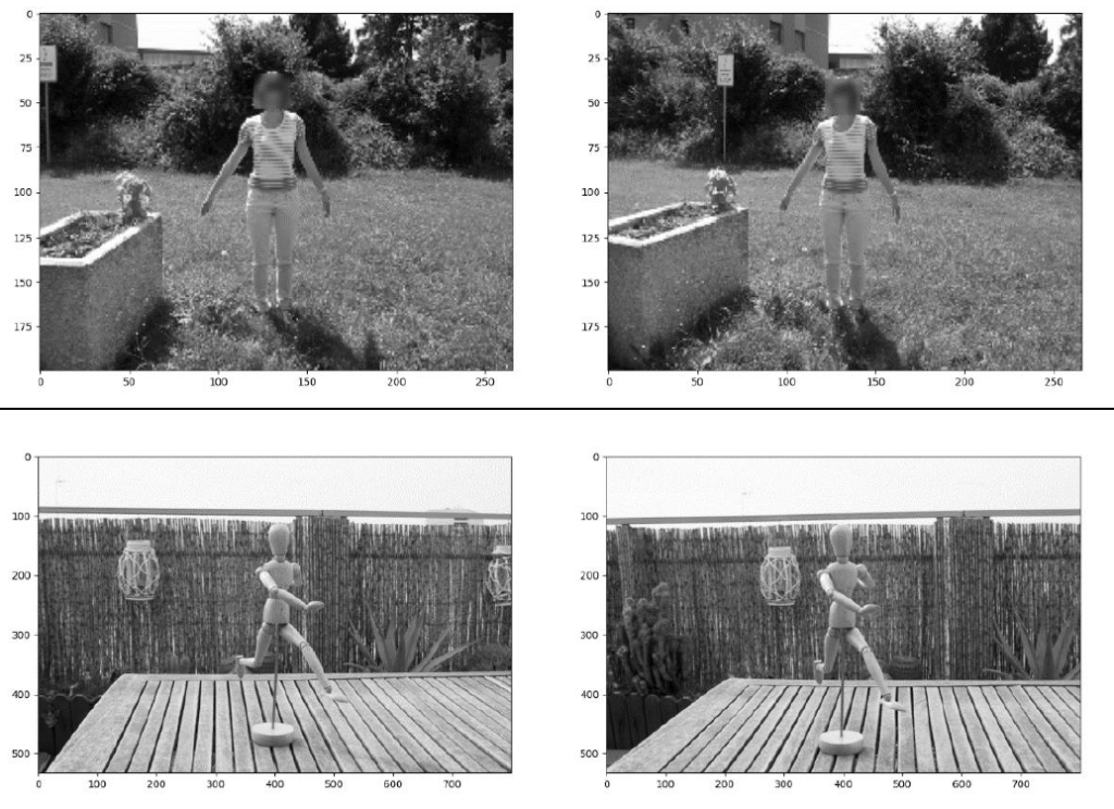
# Read both images and convert to grayscale
left_img = cv.imread('img_pair_2/image2_left.jpg', cv.IMREAD_GRAYSCALE)
right_img = cv.imread('img_pair_2/image2_right.jpg', cv.IMREAD_GRAYSCALE)

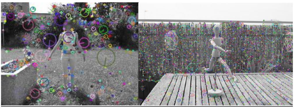
## Detecting Keypoints 
# detect SIFT keypoints and descriptors 

# Initialize SIFT detector
sift = cv.SIFT_create()
# find the keypoints and descriptors with SIFT
kp1, des1 = sift.detectAndCompute(left_img, None)
kp2, des2 = sift.detectAndCompute(right_img, None)

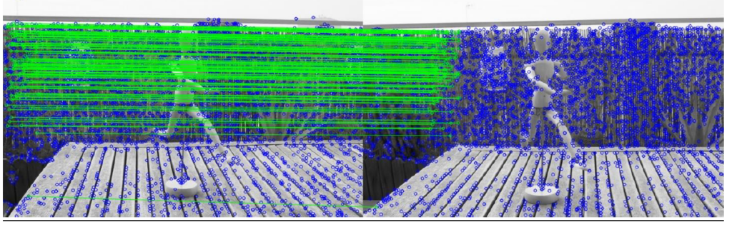
## Matching Keypoints 
# match keypoints in left and right images using FLANN matcher
flann = cv.FlannBasedMatcher(dict(algorithm=1, trees=5), dict(checks=50))
matches = flann.knnMatch(des1, des2, k=2)

# keep good matches
matchesMask = [[0, 0] for i in range(len(matches))]
good = []
pts1 = []
pts2 = []

for i, (m, n) in enumerate(matches):
    if m.distance < 0.7*n.distance:
        # Keep this keypoint pair
        matchesMask[i] = [1, 0]
        good.append(m)
        pts2.append(kp2[m.trainIdx].pt)
        pts1.append(kp1[m.queryIdx].pt)

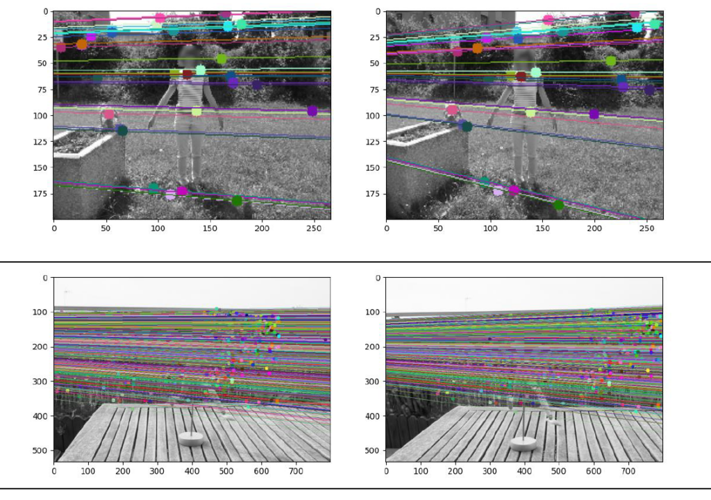
## Stereo Rectification
 
# calculate fundamental matrix using ransac
pts1 = np.int32(pts1)
pts2 = np.int32(pts2)
fundamental_matrix, inliers = cv.findFundamentalMat(pts1, pts2, cv.FM_RANSAC)

# select only inlier points
pts1 = pts1[inliers.ravel() == 1]
pts2 = pts2[inliers.ravel() == 1]


# visualize epilines

# Find epilines corresponding to points in right image (second image) and
# drawing its lines on left image
lines1 = cv.computeCorrespondEpilines(
    pts2.reshape(-1, 1, 2), 2, fundamental_matrix)
lines1 = lines1.reshape(-1, 3)
img5, img6 = drawlines(left_img, right_img, lines1, pts1, pts2)


# Find epilines corresponding to points in left image (first image) and
# drawing its lines on right image
lines2 = cv.computeCorrespondEpilines(
    pts1.reshape(-1, 1, 2), 1, fundamental_matrix)
lines2 = lines2.reshape(-1, 3)
img3, img4 = drawlines(right_img, left_img, lines2, pts2, pts1)

"""
plt.subplot(121), plt.imshow(img5)
plt.subplot(122), plt.imshow(img3)
plt.suptitle("Epilines in both images")
plt.show()
"""

# Stereo rectification from uncalibrated source
h1, w1 = left_img.shape
h2, w2 = right_img.shape
_, H1, H2 = cv.stereoRectifyUncalibrated(
    np.float32(pts1), np.float32(pts2), fundamental_matrix, imgSize=(w1, h1)
)

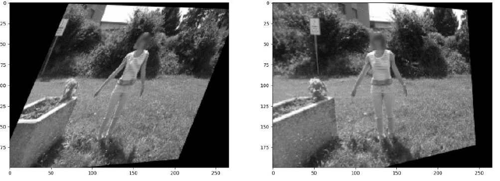
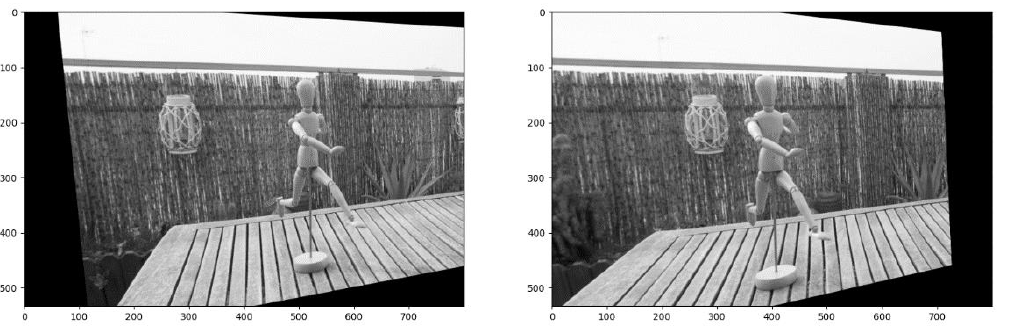
# rectify and save images
left_img_rectified = cv.warpPerspective(left_img, H1, (w1, h1))
right_img_rectified = cv.warpPerspective(right_img, H2, (w2, h2))
cv.imwrite("rectified_left.png", left_img_rectified)
cv.imwrite("rectified_right.png", right_img_rectified)

# print program execution time
print(" Program Execution Time: %s seconds" % (time.time() - start_time))

# Draw the rectified images
fig, axes = plt.subplots(1, 2, figsize=(15, 10))
axes[0].imshow(left_img_rectified, cmap="gray")
axes[1].imshow(right_img_rectified, cmap="gray")

plt.suptitle("Rectified images")
plt.savefig("rectified_images.png")
plt.show()

Table of Contents